Tiedosto:Conformal map.svg

Tämän PNG-esikatselun koko koskien SVG-tiedostoa: 342 × 599 kuvapistettä. Muut resoluutiot: 137 × 240 kuvapistettä | 274 × 480 kuvapistettä | 438 × 768 kuvapistettä | 584 × 1 024 kuvapistettä | 1 169 × 2 048 kuvapistettä | 535 × 937 kuvapistettä.
Alkuperäinen tiedosto (SVG-tiedosto; oletustarkkuus 535 × 937 kuvapistettä; tiedostokoko 34 KiB)
| Tämä tiedosto on tiedostotietokanta Wikimedia Commonsista. Tiedot kuvaussivulta näkyvät alla. |  |
Tiedoston kuvaussivu Commonsissa |
Yhteenveto
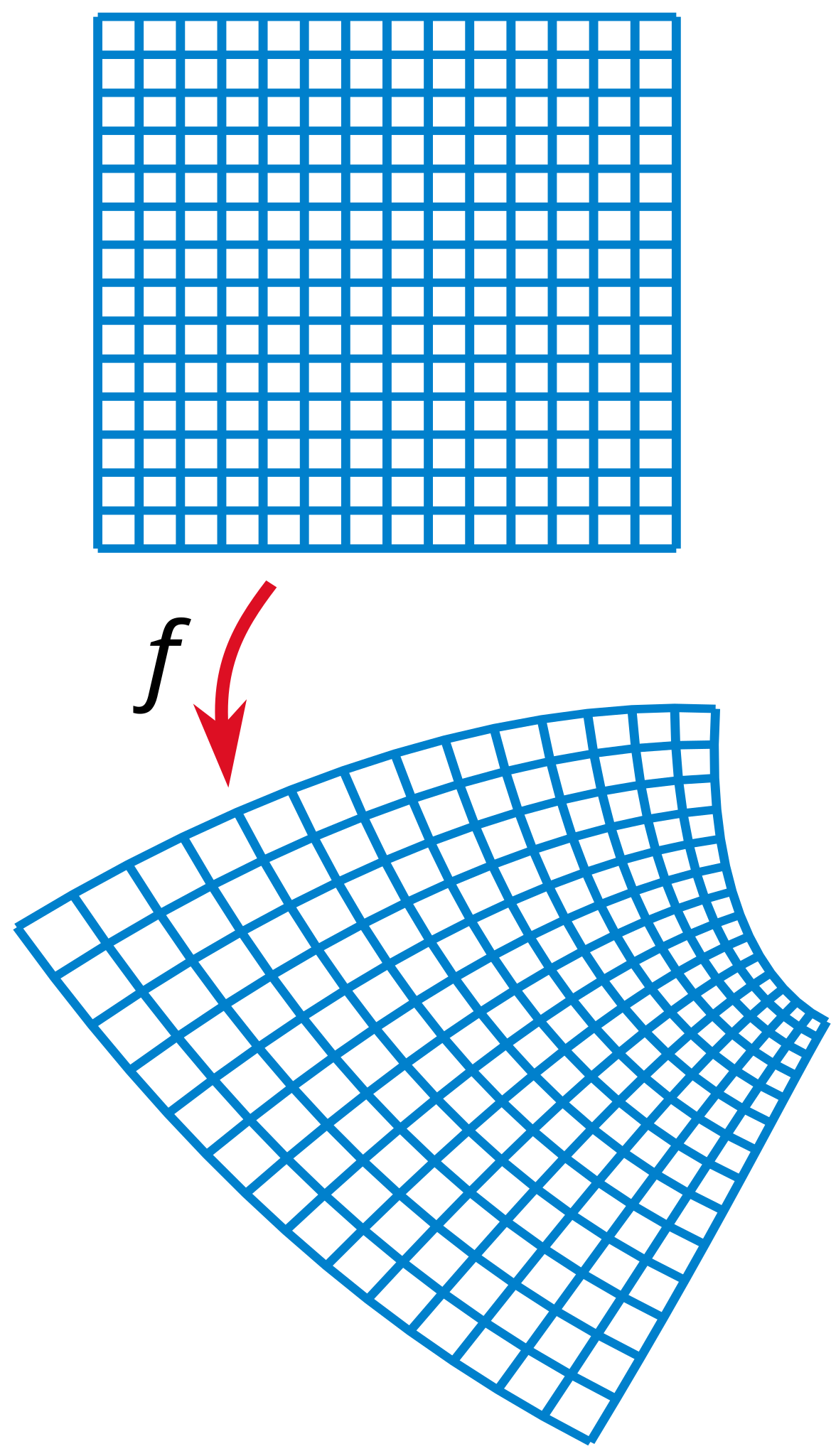
| Kuvaus | Illustration of a conformal map. |
| Päiväys | |
| Lähde | self-made with MATLAB, tweaked in Inkscape. |
| Tekijä | Oleg Alexandrov |
| SVG kehittely | Tämä vektorigrafiikkatiedosto luotiin käyttäen apuna ohjelmaa Inkscape This file uses translateable embedded text. |
Lisenssi
| Minä, tämän teoksen tekijänoikeudellinen omistaja, julkaisen tämän teoksen public domainiin eli luovun kaikista tekijänoikeuksista lain sallimissa puitteissa. Tämä on voimassa maailmanlaajuisesti. Joissain maissa laki ei mahdollista tätä. Mikäli näin on: Myönnän kenelle tahansa oikeuden käyttää tätä teosta mihin tahansa tarkoitukseen, ilman mitään ehtoja, ellei laki vaadi ehtojen asettamista. |
Source code (MATLAB)
% Compute the image of a rectangular grid under a a conformal map.

function main()

   N = 15; % num of grid points
   epsilon = 0.1; % displacement for each small diffeomorphism
   num_comp = 10; % number of times the diffeomorphism is composed with itself

   S = linspace(-1, 1, N);

   [X, Y] = meshgrid(S);


   % graphing settings
   lw = 1.0;

   % KSmrq's colors
   red    = [0.867 0.06 0.14];
   blue   = [0, 129, 205]/256;
   green  = [0, 200,  70]/256;
   yellow = [254, 194,   0]/256;
   white = 0.99*[1, 1, 1];

   mycolor = blue;

   % start plotting
   figno=1; figure(figno); clf;

   shiftx = 0; shifty = 0; scale = 1;
   do_plot(X, Y, lw, figno, mycolor, shiftx, shifty, scale)

   I=sqrt(-1);
   Z = X+I*Y;

   % tweak these numbers for a pretty map
   z0 = 1+ 2*I;
   z1 = 0.1+ 0.2*I;
   z2 = 0.2+ 0.3*I;
   a = 0.01;
   b = 0.02;
   shiftx = 0.1; shifty = 1.2; scale = 1.4;
   F = (Z+z0).^2 +a*(Z+z1).^3 +b*(Z+z2).^4;
   F = (1+2*I)*F;

   XF = real(F); YF=imag(F);

   do_plot(XF, YF, lw, figno, mycolor, shiftx, shifty, scale)

   axis ([-1 1.3 -2 2]); axis off;

   saveas(gcf, 'Conformal_map.eps', 'psc2');


function do_plot(X, Y, lw, figno, mycolor, shiftx, shifty, scale)
   figure(figno); hold on;

   [M, N] = size(X);

   X = X - min(min(X));
   Y = Y - min(min(Y));

   a = max(max(max(abs(X))), max(max(abs(Y))));
   X = X/a; Y = Y/a;

   X = scale*(X-shiftx);
   Y = scale*(Y-shifty);

   for i=1:N
      plot(X(:, i), Y(:, i), 'linewidth', lw, 'color', mycolor);
      plot(X(i, :), Y(i, :), 'linewidth', lw, 'color', mycolor);
   end
%   axis([-1-small, 1+small, -1-small, 1+small]);
   axis equal; axis off;
Tiedoston historia
Päiväystä napsauttamalla näet, millainen tiedosto oli kyseisellä hetkellä.
| Päiväys | Pienoiskuva | Koko | Käyttäjä | Kommentti | |
|---|---|---|---|---|---|
| nykyinen | 28. tammikuuta 2008 kello 00.51 | | 535 × 937 (34 KiB) | Oleg Alexandrov | Make arrow and text smaller |
| 23. tammikuuta 2008 kello 06.36 |  | 535 × 937 (34 KiB) | Oleg Alexandrov | {{Information |Description=Illustration of a conformal map. |Source=self-made with MATLAB, tweaked in Inkscape. |~~~~~ |Author= Oleg Alexandrov |Permission= |other_versions= }} {{PD-self}} ==Source code ([[ |
Tiedoston käyttö
Seuraavat 2 sivua käyttävät tätä tiedostoa:
Tiedoston järjestelmänlaajuinen käyttö
Seuraavat muut wikit käyttävät tätä tiedostoa:
- Käyttö kohteessa ar.wikipedia.org
- Käyttö kohteessa ba.wikipedia.org
- Käyttö kohteessa ca.wikipedia.org
- Käyttö kohteessa cbk-zam.wikipedia.org
- Käyttö kohteessa cs.wikipedia.org
- Käyttö kohteessa de.wikipedia.org
- Käyttö kohteessa de.wikiversity.org
- Holomorphie/Kriterien
- Kurs:Riemannsche Flächen (Osnabrück 2022)/Vorlesung 1
- Kurs:Riemannsche Flächen (Osnabrück 2022)/Vorlesung 1/kontrolle
- Satz über die Umkehrabbildung/Implizite Abbildung/C/Zusammenfassung/Textabschnitt
- Kurs:Funktionentheorie (Osnabrück 2023-2024)/Vorlesung 4
- Kurs:Funktionentheorie (Osnabrück 2023-2024)/Vorlesung 4/kontrolle
- Käyttö kohteessa el.wikipedia.org
- Käyttö kohteessa en.wikipedia.org
- Käyttö kohteessa es.wikipedia.org
- Käyttö kohteessa fa.wikipedia.org
- Käyttö kohteessa fr.wikipedia.org
- Käyttö kohteessa gl.wikipedia.org
- Käyttö kohteessa he.wikipedia.org
- Käyttö kohteessa hi.wikipedia.org
- Käyttö kohteessa hu.wikipedia.org
- Käyttö kohteessa hy.wikipedia.org
- Käyttö kohteessa id.wikipedia.org
- Käyttö kohteessa it.wikipedia.org
- Käyttö kohteessa ja.wikipedia.org
Näytä lisää tämän tiedoston järjestelmänlaajuista käyttöä.